Full Employment Output

View FREE Lessons!

Definition of Full Employment Output:

An economy’s full employment output is the production level (RGDP) when all available resources are used efficiently. It equals the highest level of production an economy can sustain for the long run. It is also referred to as the full employment production, natural level of output, or long-run aggregate supply. 

Detailed Explanation:

An economy’s full employment output is its maximum sustainable output. The economy is at full employment when all the factors of production, including labor, are being used efficiently but not stretched beyond their capacity. Graphically it is where the long-run aggregate supply intersects with the x-axis on the graph below. 

Graph 1


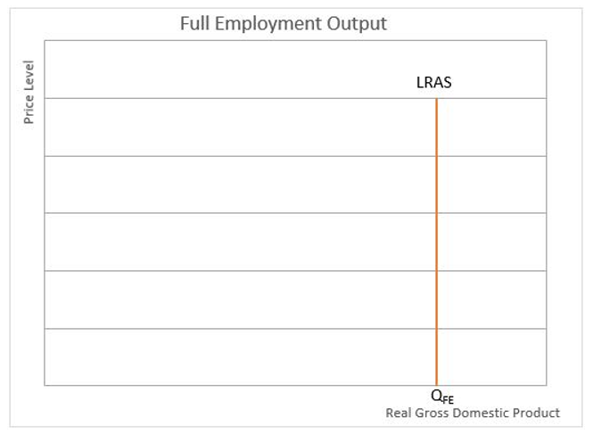
Why is the long-run aggregate supply curve (LRAS) vertical? Economists refer to the long run when they assume all prices and inputs are flexible. This includes input prices such as labor and raw materials as well as the prices of final goods and services. In the long run, an economy’s potential is limited by its factors of production which include its natural resources, people, technology, entrepreneurs, and capital. Note that the price is not mentioned. In the long run, production is independent of the price level. In other words, whether the price level increases or decreases, the full employment RGDP is unchanged.

Why is the full employment output independent of the price level? 

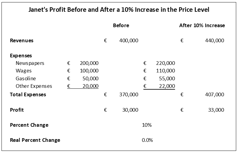
Production is driven by profits, so we must show that profits do not increase in the long run following an increase in the price level to prove long-run production is independent of the price level.

The French company, Janet’s Newspaper Delivery Service illustrates this point. Assume inflation is ten percent, so Janet increases her price by ten percent. The cost of her papers, employees’ wages, rent, gasoline, and all other costs also increase by the general price level, or ten percent. The table below shows the resulting profits before and after the increase in the price level. Janet’s profit increases ten percent, but she is no better off than before because all the prices in the economy have increased ten percent. Her purchasing power is unchanged. Therefore, there is no incentive for Janet to increase her supply i.e. the number of papers she sells. If we extend this specific example to every business in every sector of the economy, we can understand why when all prices increase or decrease by the same percentage, the full employment output is unaffected. 



How does an economy return to the full employment output when the economy is in a recession?

Prices and output are flexible in the long run. When something triggers a drop in the economy’s aggregate demand, the price level, and short-term output fall – until the prices of all inputs and outputs adjust. Assume a financial crisis lowers the demand for Janet’s delivery service and she is forced to lower her prices ten percent. Initially, she is very reluctant to decrease the amount she pays her employees, and gasoline prices remain unchanged. Profits decline, so she is willing to supply fewer newspapers at the lower price. However, in the long run, prices and wages adjust. Some employees may accept a ten percent reduction in pay. Others may be let go since she sells fewer newspapers. Gasoline prices match the ten percent decline in the price level. The reduction in her costs boosts profits so she is again willing to provide the same number of newspapers as before. The economy has returned to the full employment level of production, but at a lower price level. This is illustrated with the series of graphs below.

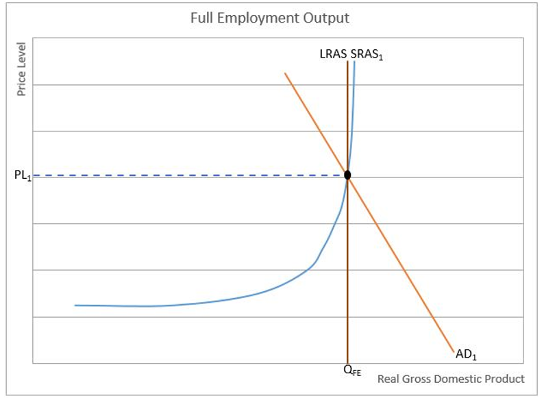
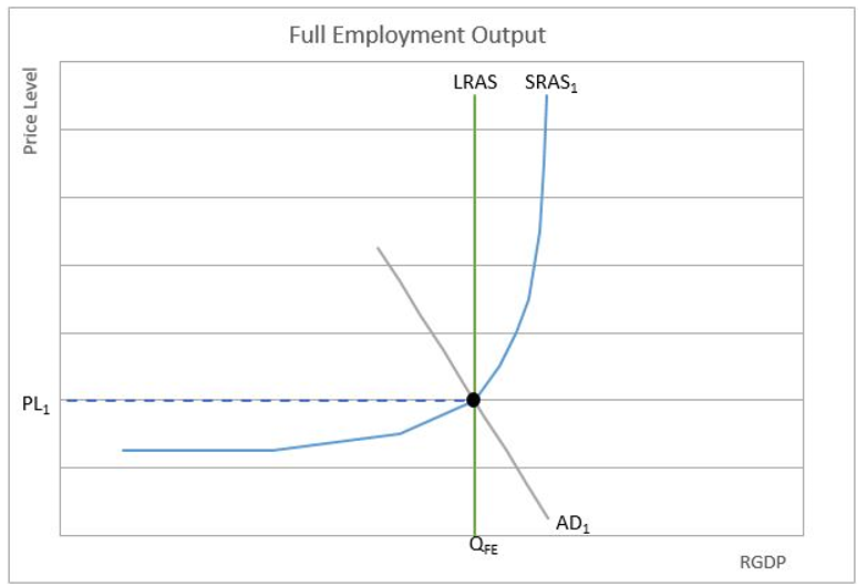
Initially, the economy is operating in a long-run equilibrium where the short-run aggregate supply (SRAS), LRAS, and aggregate demand (AD) are in equilibrium and the resulting price level is PL₁ and Q_FE is the RGDP.

Graph 2A


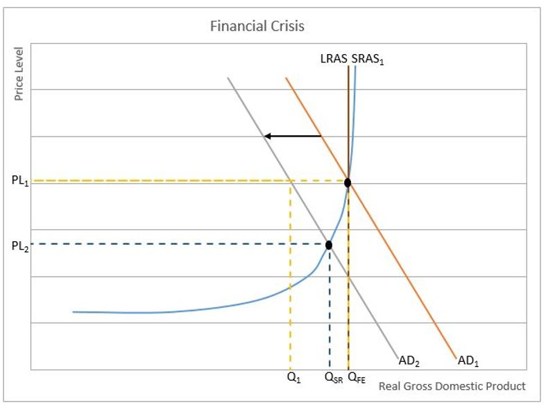
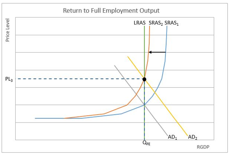
Assume a financial crisis triggers a drop in the aggregate demand from AD₁ to AD₂, as shown in Graph 2B. Shortly after, companies see the demand for their goods and services decrease. Output would fall to Q₁ if the price level remained at PL₁, but companies respond by lowering their prices hoping to increase the quantity demanded for the good or service they offer. Because they are unable to reduce all their costs, production still falls, but not to the same degree as it would without reducing prices. In the short run, there is movement along the SRAS from (PL₁, Q_FE) to (PL₂, Q_SR). A short-term equilibrium is reached where the price level is PL₂ and production falls to Q_SR. 

Graph 2B


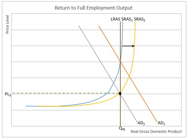
At this point, some employees have lost their jobs, and the demand for other inputs has decreased because production in the economy has fallen. All producers are benefiting from a lower cost because the decrease in demand for inputs has resulted in a lower input cost, which causes a rightward shift of the economy's short-run aggregate supply curve to SRAS₂. Employees are rehired, but at a lower wage, which in theory they do not mind since the economy’s price level has also decreased. In the long run all prices in the economy decrease by the same percentage. Eventually, long-run equilibrium is reached where the output returns to the full employment equilibrium, Q_FE, and the price-level drops to PL₃. This illustrates how an economy recovers and returns to its full employment output following a financial crisis. 

Graph 2C


How does an economy return to its full employment output when the economy overheats? 

When an economy is operating at its long-run equilibrium all resources are being used at the full employment or natural production rate. Resources are not pushed beyond the point where prices are dramatically impacted. Full employment does not mean there is no unemployment. Some workers take advantage of the tight labor market and seek advances. Economists differ in their views on what the full employment rate is, but most agree it is between 95 and 97 percent. 

Economies can be compared to long-distance runners. Long-distance runners are most efficient when they pace themselves. They can sprint for short periods but tire and ultimately hurt their performance if they do so for too long. Like long-distance runners, an economy is most efficient when it paces itself. For short periods, an economy can operate beyond its long-run aggregate supply. Economists use similar terms such as “tired,” “overheated,” and “spent” to describe an economy in this phase. During these periods, manufacturers may defer maintenance to continue meeting demand. Workers may tire and become less productive when working overtime for extended periods. Companies raise prices to reduce their quantity demanded. Initially, profits rise, but in the long-run wages will increase because the demand for workers has increased and employees work overtime. Raw materials have also become more expensive because of mounting demands. Eventually, the price of all inputs increases. The higher costs return profits to normal and output is cut back to the full employment output, but the price level has increased. This is illustrated in steps on the graphs below.  

Let us return to when the economy is operating in long-run equilibrium. The short-run aggregate supply (SRAS), LRAS, and aggregate demand (AD) are in equilibrium and the resulting price level is PL₁ and Q_FE is the RGDP. 

Graph 3A


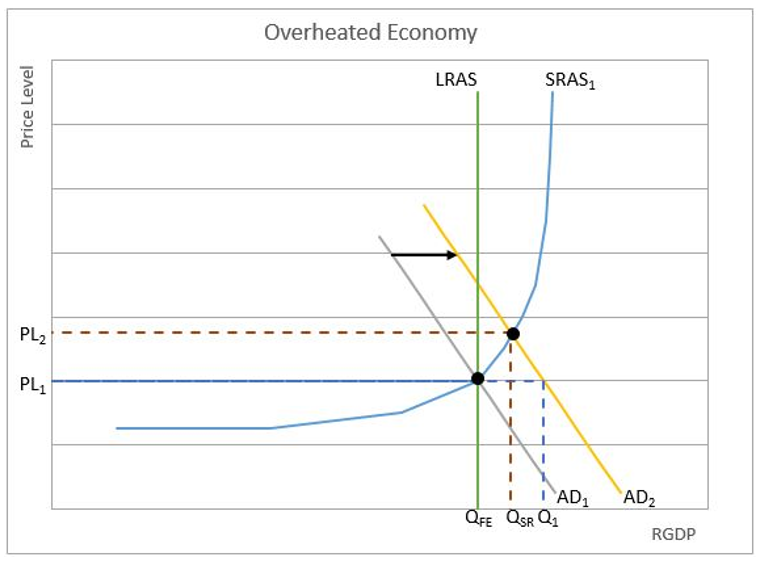
Assume an overheated economy increases the aggregate demand from AD₁ to AD₂. Shortly after, companies see the demand for their goods and services increase. Output would increase to Q₁ if the price level remained at PL₁, but companies respond by increasing their prices hoping to take advantage of the increase in demand. However, their marginal costs are also increasing. In the short run, there is movement along the SRAS from (PL₁, Q_FE) to (PL₂ Q_SR). Companies increase production and increase their prices to meet the increase in demand. Short-run equilibrium is reached where the price level is PL₂ and production increases to Q_SR.

Graph 3B


At this point, employees are working overtime and more are being hired. Suppliers are having trouble meeting the company’s increased demand. The forces of an increase in demand and decrease in the available supply of inputs have pushed the production cost higher, which shifts the short-run aggregate supply curve (SRAS) to the left, to SRAS₂. Eventually, a new long-run equilibrium is reached, resulting in the same production as before, Q_FE, but a higher price level, PL₃. This illustrates how an economy cannot sustain production beyond its full employment output.

Graph 3C

Dig Deeper With These Free Lessons:

Aggregate Supply and Demand – Macroeconomic Equilibrium
Aggregate Supply – Relating Inflation and Production
Fiscal Policy – Managing an Economy by Taxing and Spending
Factors of Production – The Required Inputs of Every Business